Determining the Number of Clusters: A Comprehensive Guide

Clustering, a fundamental technique in unsupervised machine learning, involves grouping similar data points together. It has diverse applications, including customer segmentation, image processing, and anomaly detection. One of the most critical and challenging aspects of clustering is determining the number of clusters in your data. In this comprehensive guide, we will explore various methods and techniques, including prediction strength and co-membership matrix, to help you make an informed decision about the optimal number of clusters for your dataset.
Why is Choosing the Right Number of Clusters Important?
The quality and interpretability of your clustering results are strongly impacted by the number of clusters you choose, therefore choosing the right number is essential. You run the danger of oversimplifying the underlying structure of your data if you select too few clusters, which could lead to the loss of significant patterns or groups. On the other hand, choosing an excessive number of clusters might result in overfitting, when the model identifies patterns that are difficult to extrapolate to fresh data.
Methods for Determining the Number of Clusters
1. The Elbow Method:
- The elbow method is one of the most commonly used techniques for determining the number of clusters.
- It involves running the clustering algorithm with different numbers of clusters and calculating the within-cluster sum of squares (WCSS) for each number.
- Mathematically, WCSS is computed as follows:

where k is the number of clusters, nᵢ is the number of data points in cluster i, xⱼ is a data point in cluster i, and μᵢ is the centroid of cluster i.
- The idea is to look for the “elbow point” on the graph, where the rate of decrease in WCSS starts to slow down.
- The number of clusters at the elbow point is often considered a reasonable choice.
Python Packages for Clustering Analysis:

To implement these techniques and perform clustering analysis in Python, you
can use various libraries and packages:

- **scikit-learn:** This popular machine learning library provides tools for
clustering, including K-Means, hierarchical clustering, and spectral clustering
. You can also calculate the Silhouette Score and use cross-validation
techniques.

```python
# Sample code using scikit-learn for K-Means clustering and Silhouette Score
from sklearn.cluster import KMeans
from sklearn.metrics import silhouette_score
from sklearn.datasets import make_blobs

# Generate sample data
X, _ = make_blobs(n_samples=300, centers=4, random_state=2)

# Determine the optimal number of clusters using the Elbow method
wcss = []
for i in range(1, 11):
    kmeans = KMeans(n_clusters=i, init='k-means++', max_iter=300, n_init=10, random_state=2)
    kmeans.fit(X)
    wcss.append(kmeans.inertia_)

# Plot the Elbow method
import matplotlib.pyplot as plt
plt.plot(range(1, 11), wcss)
plt.title('Elbow Method')
plt.xlabel('Number of clusters')
plt.ylabel('WCSS')  # Within-cluster sum of squares
plt.show()

# Choose the number of clusters based on the Elbow method
optimal_num_clusters = 4  # In this example, it would be chosen based on the plot
print(f'Optimal number of clusters: {optimal_num_clusters}')

# Perform K-Means clustering with the chosen number of clusters
kmeans = KMeans(n_clusters=optimal_num_clusters, init='k-means++', max_iter=300, n_init=10, random_state=2)
kmeans.fit(X)

# Calculate the Silhouette Score
silhouette_avg = silhouette_score(X, kmeans.labels_)
print(f'Silhouette Score: {silhouette_avg}')
2. The Silhouette Score:
- The silhouette score measures how similar an object is to its own cluster compared to other clusters.
- Mathematically, the silhouette score for a data point x is computed as:

- where a(x) is the average distance from x to the other data points in the same cluster, and b(x) is the minimum average distance from x to data points in a different cluster.
- A higher silhouette score indicates that the object is well-matched to its cluster.
3. Gap Statistics:
- Gap statistics compare the performance of your clustering algorithm on the actual data to its performance on random data (generated under the assumption of no meaningful clusters).
- Mathematically, gap statistics involve comparing the observed within-cluster sum of squares to the expected within-cluster sum of squares under a null hypothesis.
4. Dendrogram Analysis:
- A dendrogram is a tree-like diagram that shows the hierarchical relationships between clusters. It is created by a clustering algorithm, which starts by treating each data point as a separate cluster. The algorithm then repeatedly merges the two closest clusters until there is only one cluster left. The dendrogram shows the order in which the clusters were merged.
- The branches of a dendrogram represent the distances between clusters. The closer the two branches are, the more similar the two clusters are. The point where the branches start to merge less rapidly is the point where the clusters are becoming more distinct.
- The number of clusters at this point can be a reasonable estimate of the number of clusters in the data. However, it is important to note that this is just an estimate, and the actual number of clusters may vary depending on the clustering algorithm and the data set.
5. Prediction Strength and Co-Membership Matrix:
- Prediction Strength (PS) assesses the stability of the clusters by repeatedly subsampling the data and clustering subsets of it.
- It measures how often data points that belong to the same cluster in the original data are still clustered together in the subsamples.
- A higher Prediction Strength indicates more stable and robust clusters.
To calculate Prediction Strength, follow these steps {N has been subscripted as “ₙ” in text}:
a. Randomly subsample your data N times to create N subsets, denoted as D₁,D₂,…,Dₙ.
b. Apply the clustering algorithm to each subset Di to obtain N sets of clusters, denoted as C₁,C₂,…,Cₙ.
c. For each subset Dᵢ, create a co-membership matrix Mᵢ that quantifies how often pairs of data points are assigned to the same cluster across the N runs of clustering. The co-membership matrix Mᵢ is a binary matrix where Mᵢⱼ=1 if data points i and j belong to the same cluster in at least one of the N runs, and Mᵢⱼ=0 otherwise.
d. Aggregate the N co-membership matrices M₁,M₂,…,Mₙ into a consensus co-membership matrix M꜀ₒₙₛₑₙₛᵤₛ.
e. The Prediction Strength PS for a pair of data points i and j is calculated as:
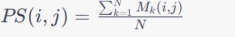
f. A higher aggregated Prediction Strength suggests more stable clusters, indicating that the chosen number of clusters is robust.
To explain it in simpler terms, Prediction Strength is like a test that checks how well a group of data points (the “test data”) consistently sticks together in the same cluster after we’ve trained a clustering model on another group of data points (the “train data”). It helps us see if the clusters are reliable.
Imagine you have a collection of colored marbles (your data points), and you want to group them by color (create clusters). You take some of the marbles (train data), mix them up, and put them into separate boxes (clusters) based on their colors. Now, you want to know if the boxes are good at keeping marbles of the same color together.
So, you take a different set of marbles (test data), shuffle them up, and also put them into the boxes (clusters) using the same rules as before. Prediction Strength tells you how often the marbles of the same color end up in the same box (cluster) when you do this with different sets of marbles (test data).The higher the Prediction Strength, the more confident you can be that your clusters are reliable. It means that no matter which marbles you pick, the boxes (clusters) consistently group them correctly by color.
The Co-Membership Matrix is like a record of which marbles (data points) often end up in the same box (cluster) when we do the grouping (clustering) multiple times with different sets of marbles (test data).
Imagine you have a chart with all the marbles on one side and boxes (clusters) on the other. Each cell in the chart shows how many times two marbles (data points) were put in the same box (cluster) when you did the clustering with different sets of marbles (test data). If a cell has a high number, it means those two marbles are often put in the same box (cluster) together, which suggests they belong together. If the number is low, it means they don’t usually end up in the same box (cluster).
By looking at this chart (the Co-Membership Matrix), you can get a sense of how strongly related the marbles (data points) are to each other when forming clusters, helping you decide how many clusters are meaningful in your data. So, Prediction Strength and the Co-Membership Matrix are tools to check how well your clusters work and how stable they are when you try different sets of data.
Python Packages for Clustering Analysis:
To implement these techniques and perform clustering analysis in Python, you can use various libraries and packages:
- scikit-learn: This popular machine learning library provides tools for clustering, including K-Means, hierarchical clustering, and spectral clustering. You can also calculate the Silhouette Score and use cross-validation techniques.
- gap-statistics: The
gap-statisticspackage offers functions to compute gap statistics, which can help you determine the number of clusters using the gap statistic method.
You can refer to this paper for more information,
“Estimating the Number of Clusters in a Data Set Via the Gap Statistic”
https://hastie.su.domains/Papers/gap.pdf
# Sample code using the gap-statistics package
from gap_statistic import OptimalK
import numpy as np

# Generate sample data
X = np.random.rand(300, 2)

# Compute optimal number of clusters using the gap statistic
optimalK = OptimalK(parallel_backend='joblib')
n_clusters = optimalK(X, cluster_array=np.arange(1, 11))

print(f'Optimal number of clusters: {n_clusters}')- SciPy: SciPy provides tools for hierarchical clustering and dendrogram analysis. You can use the
dendrogramfunction to visualize dendrograms and identify the optimal number of clusters.
# Sample code using SciPy for hierarchical clustering and dendrogram visualization
from scipy.cluster.hierarchy import dendrogram, linkage
import matplotlib.pyplot as plt
import numpy as np

# Generate sample data
X = np.random.rand(10, 2)

# Perform hierarchical clustering
linked = linkage(X, 'ward')

# Plot the dendrogram
dendrogram(linked, orientation='top', distance_sort='descending', show_leaf_counts=True)
plt.title('Hierarchical Clustering Dendrogram')
plt.xlabel('Sample Index')
plt.ylabel('Distance')
plt.show()- yellowbrick: The
yellowbricklibrary offers a range of visualizations, including the elbow method, silhouette plots, and more, to assist in choosing the right number of clusters.
# Sample code using yellowbrick for the elbow method
from yellowbrick.cluster import KElbowVisualizer
from sklearn.cluster import KMeans

# Generate sample data
X, _ = make_blobs(n_samples=300, centers=4, random_state=42)

# Instantiate the KElbowVisualizer with the KMeans clustering model
model = KMeans()
visualizer = KElbowVisualizer(model, k=(1,11))

# Fit the visualizer to the data and visualize the elbow method plot
visualizer.fit(X)
visualizer.show()- scipy.cluster.hierarchy: For hierarchical clustering, you can use the
scipy.cluster.hierarchymodule, which is part of the SciPy library. - numpy: You can use NumPy for various numerical operations and to perform matrix manipulations required for co-membership matrix and Prediction Strength calculations.
# Sample code for Prediction Strength using a co-membership matrix
import numpy as np
from sklearn.cluster import KMeans
from sklearn.datasets import make_blobs

# Generate sample data
X, _ = make_blobs(n_samples=300, centers=4, random_state=42)

# Define the number of clusters and subsampling iterations
num_clusters = 4
num_iterations = 10

# Initialize variables to store co-membership matrices
co_membership_matrices = []

# Perform subsampling and clustering to create co-membership matrices
for _ in range(num_iterations):
    # Randomly subsample the data
    subsample_indices = np.random.choice(len(X), len(X))
    X_subsampled = X[subsample_indices]

    # Perform K-Means clustering
    kmeans = KMeans(n_clusters=num_clusters, random_state=42)
    labels = kmeans.fit_predict(X_subsampled)

    # Create a co-membership matrix for the current iteration
    co_membership_matrix = np.zeros((len(X), len(X)))
    for i in range(len(X)):
        for j in range(i + 1, len(X)):
            if labels[i] == labels[j]:
                co_membership_matrix[i, j] = 1
                co_membership_matrix[j, i] = 1

    co_membership_matrices.append(co_membership_matrix)

# Aggregate the co-membership matrices into a consensus co-membership matrix
consensus_co_membership_matrix = np.mean(co_membership_matrices, axis=0)

# Define a threshold for co-membership to consider data points in the same cluster
co_membership_threshold = 0.5  # Adjust as needed based on your data and requirements

# Calculate Prediction Strength
prediction_strength = np.mean(consensus_co_membership_matrix > co_membership_threshold)

print(f'Prediction Strength: {prediction_strength}')
In this code example, we generate a sample dataset, perform subsampling, apply K-Means clustering, and create co-membership matrices for multiple iterations. We then aggregate these matrices into a consensus co-membership matrix and calculate the Prediction Strength based on a specified co-membership threshold.
Adjust the number of clusters, subsampling iterations, and the co-membership threshold according to your dataset and requirements. The higher the Prediction Strength, the more stable and robust your clusters are.
In summary, determining the number of clusters is a critical step in the clustering process. A combination of mathematical techniques and Python packages can help you make an informed decision. It’s essential to remember that the choice of the number of clusters may evolve as you gain more insights into your data or as your business requirements change. Regularly revisiting and reevaluating your clustering solution can lead to more accurate and meaningful results, ultimately benefiting your data-driven decisions and applications.
So that’s some of the ways in which we can determine what number of clusters are sufficient for our data points.
Thanks for your time!